Tutorial on extracting the mountainous areas using QGIS + GRASS + r.neighbors using PANS OPS criteria in DOC 8168 VOL II
After the initial explanation on what mountainous terrain is and how you do the calculation for one single point for instrument flight procedure design according to PANS OPS DOC 8168 Volume II in our previous blog post, it is time to extend this concept for the complete DTM, however due to computation limits on our machine we will do smaller bits of 1 deg x 1 deg that we can later merge to cover the whole area.
We are assuming you already have QGIS installed and have a basic knowledge on how to use it. There are several online tutorials online that can be followed online like this one from qgistutorials but if you are looking for aviation specific training we recommend you contact Managed-AIS, they provide training on aeronautical charting but have an Intro to Aviation to GIS course that provides a QGIS introduction focused on aviation tasks. You can check more about Managed-AIS training offering here
Disclaimer: Introduction to GIS for Aviation course is prepared as a collaboration with M-AIS.
Also, you can use whatever DTM terrain you have and meets your requirements, you will just need to adjust the different parameters accordingly and consider the more accurate your terrain the more intense computational resources will be needed to process it. We are using SRTM 90 which has been filled for voids and downloaded from CGIAR download website since they have done additional job to enhance it, SRTM 30 m resolution is now available worldwide also but for this tutorial we will stick to SRTM 90.
This tutorial was done on an intel i5 11400 machine with 16 GB RAM so nothing out of the extraordinary, better machines will definitely be able to handle more load and the need to subdivide the tasks into smaller areas is greatly reduced.
The key part of the calculation is the use of raster processing functions which in QGIS are supplied by GRASS which is another open source software, specifically we are going to be using r.neighbors. The documentation is not so nice visually but basically what it does is that it will calculate for each raster pixel the value we want using the number of pixels we require to estimate it. If you are using ESRI ArcGIS you will need to adapt to procedures to use focal statistics and you will require to have Spatial or Image analyst license which is an additional cost.
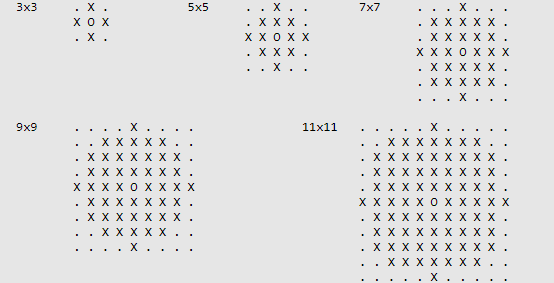
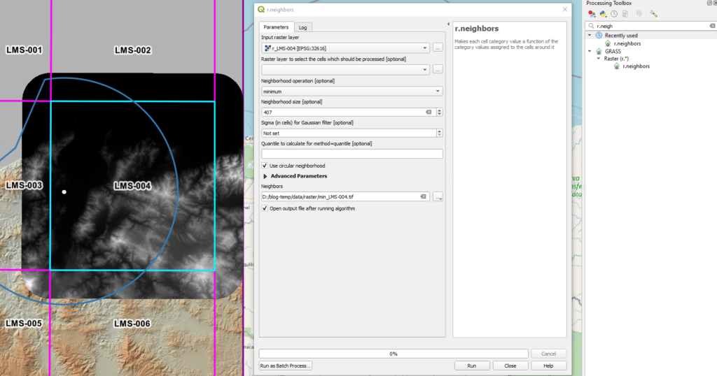
Since we know our SRTM 90 DTM has approximately 91 m per pixels in our projected coordinate system (we can get this from the DTM properties) we can estimate the number of pixels by dividing (10NM*1852m/NM)/91m=203.5 pixels but we need the diameter within r.neighbors so multiplied by 2 that gives us 407 px.
When we get to use r.neighbors this is the value we will use and the number of pixels always needs to be an odd number
We are going to start by opening QGIS and install MMQGIS plugin, this will allow us to draw our 1deg x 1deg
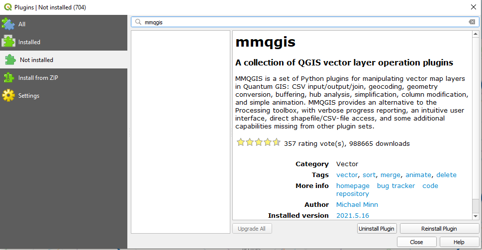
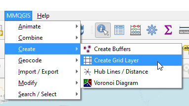
Once installed we will go to the MMQGIS menu, click on Create and then select Create Grid Layer
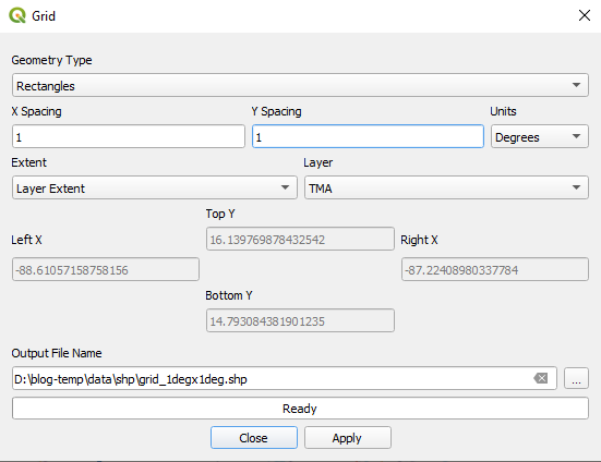
Once selected the option, we are going to change the different option to match the following in order to get a 1 degree x 1 degree grid for our study area, be careful when doing the selections as sometimes when you select something the other parameters change. Save it to somewhere in your disk with a name you will remember
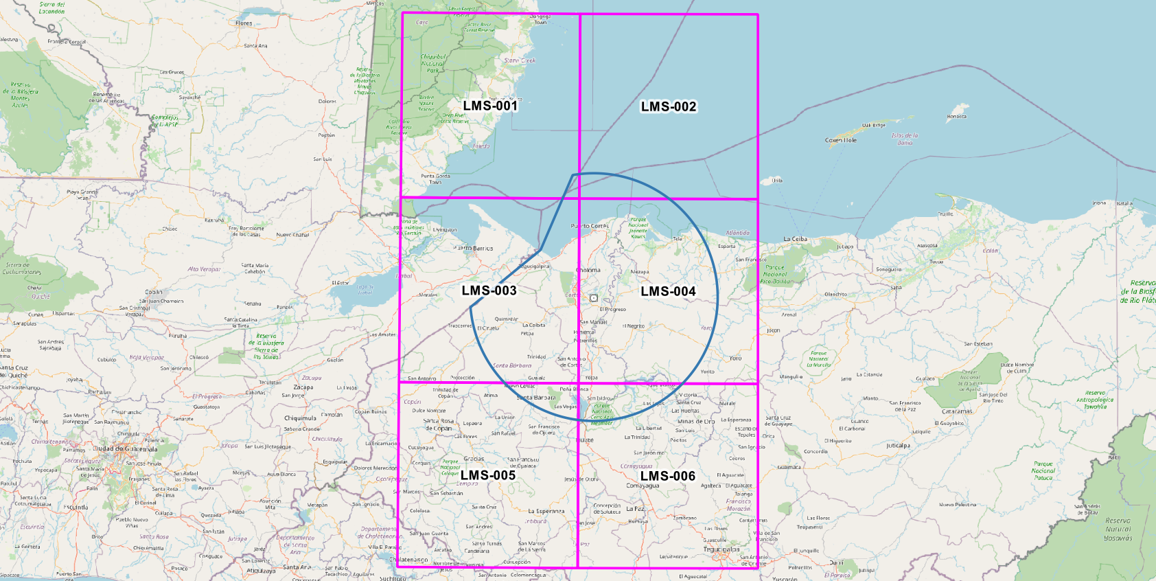
We are going to get the following grid

To keep tabs on the different blocks we will remove all columns and add a field with the following parameters that will contain a unique primary key
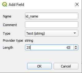
For the unique primary key we chose LMS-NNN where LMS is La Mesa (TMA NAME) and NNN is a consecutive number that will not repeat, we could have done HND for Honduras instead but for this post this will be OK as we did not generate the grid for the whole country
This process could be further automated by using model processing; however, we want to have certain quality control over the output as we progress and as we will do this once for the DTM and it can be reused then the time spent initially will be offset in the future especially since we will be having a more accurate model of where the mountainous areas are located.
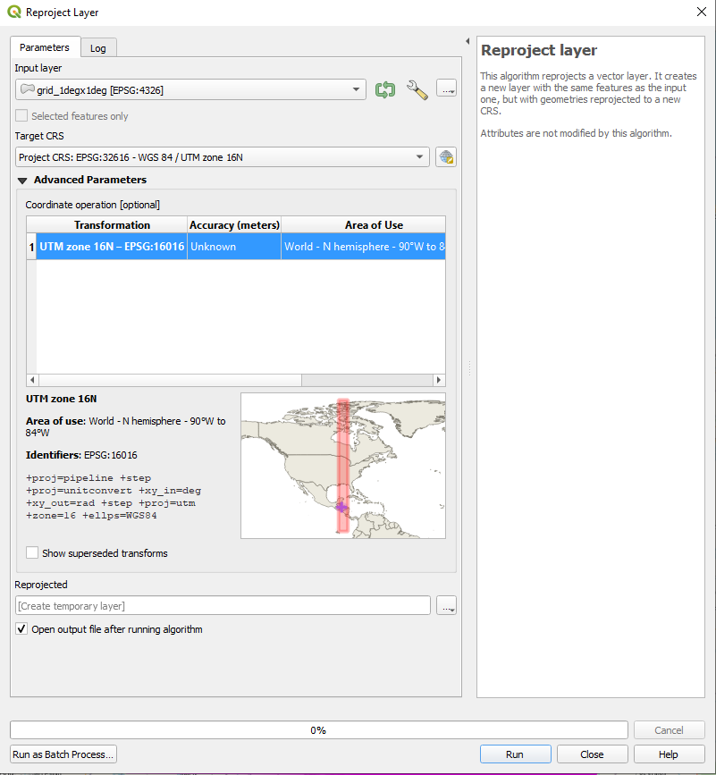
We will extract the DTM required for these tiles, first we need to reproject our grid to our projected coordinate system which in the case of Honduras is UTM 16N (EPSG 32616), we do not need a permanent layer as this is just an intermediate step
The reprojected layer we will extract the Minimum Bounding Geometry using the Bounding Box option
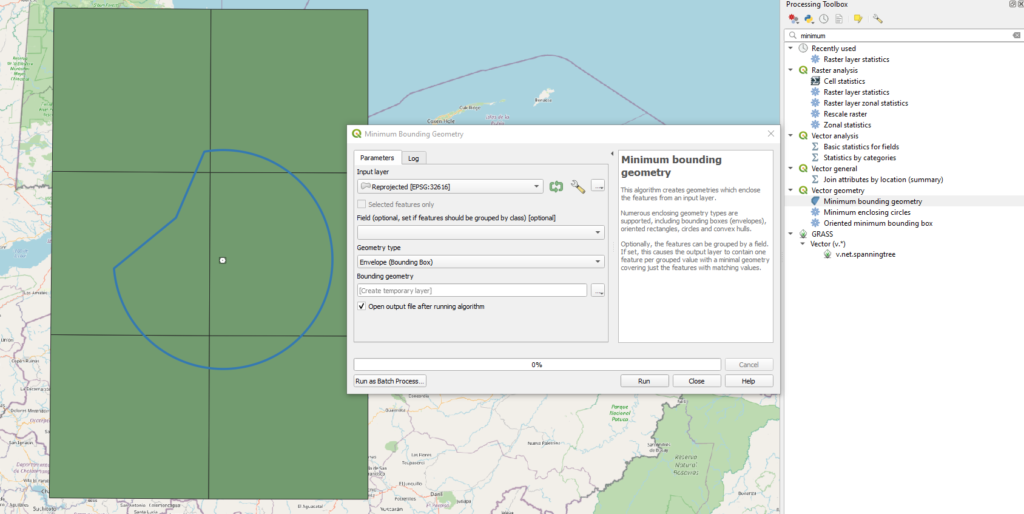
We will make a 10 NM buffer (18520m), currently QGIS has no option of using directly Nautical Miles but you can right the conversion directly in the field and it gets calculated, for example 10*1852
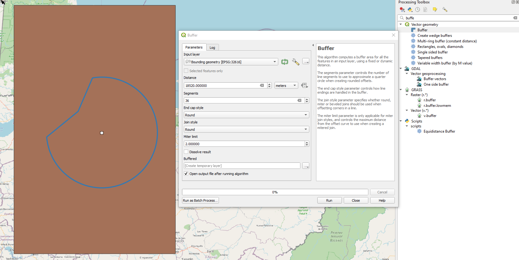
We could use the result directly but in order to get a nice rectangle cutter for our DTM we will run again the minimum bounding geometry on this last temporary file and save as grid_1degx1deg_10NM_buffer. This will be used to extract the required part of the DTM for our terrain analysis.
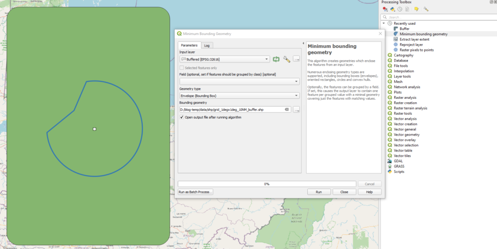
The bounding box result
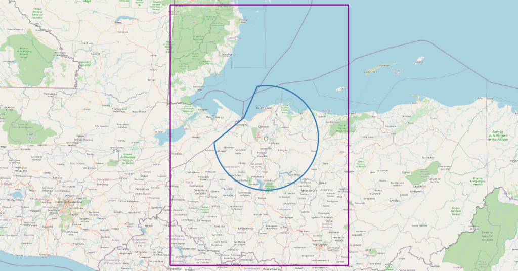
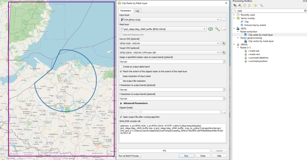
Extract the raster using the Clip Raster by Mask Layer tool from geoprocessing with the following parameters, we will not save to disk yet as we will use later the raster calculator to eliminate negative values
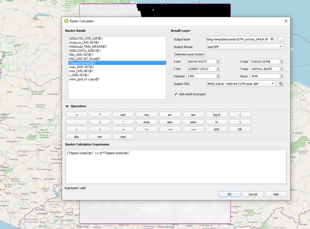
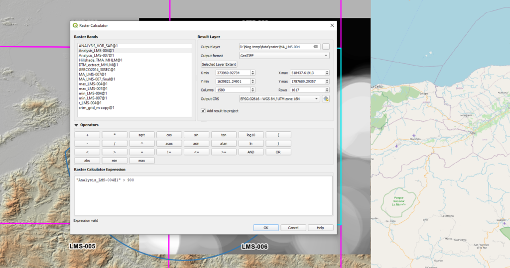
Run the raster calculator using the following values (if your country has negative elevations this might not be appropriate), in our case we want to remove the no data encoding of -32767 to 0
This is how everything looks with color ramp applied and Hillshade used, we can see the 1degx1deg tile plus the 10 NM buffer which will allow us to do the calculations valid for each tile
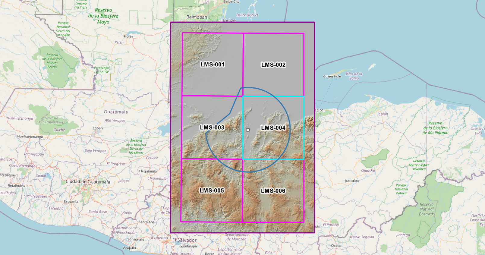
Demonstration for LMS-004
We will use LMS-004 for the demonstration. The algorithm we will be using is the following:
- We will reproject all of our tiles first to the projected coordinate system, notice the Selected features only checkbox is not active so even though we have on tile selected it will perform the operation over the complete layer.
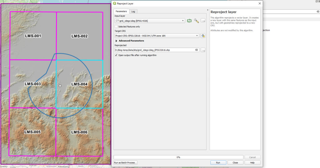
- Select the 1degx1deg tile.

- Create a 10NM buffer around it and name the file b_LMS-NNN where NNN will match the tile selected. For this reason we reprojected the grid to a projected coordinate system and use buffer operations with 18520 m (10 NM).
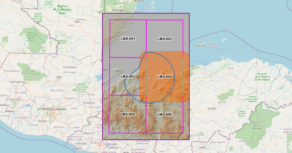
- Extract the raster using a mask to only have the DTM of the tile + 10 NM buffer using the b_LMS-004 feature created in the previous step save as r_LMS-004
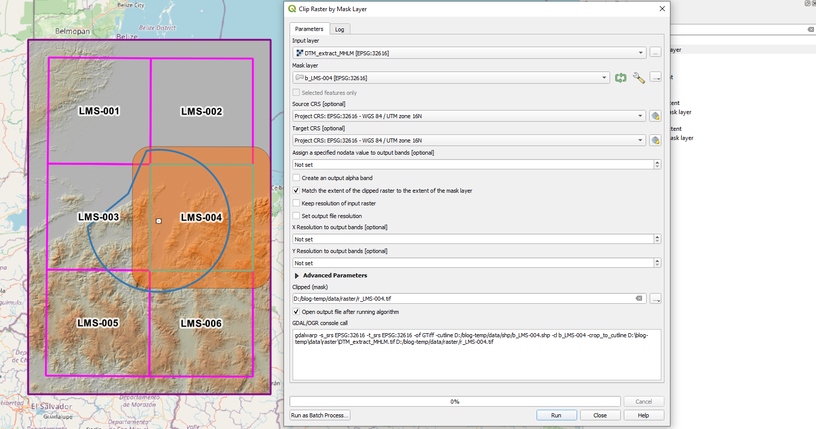
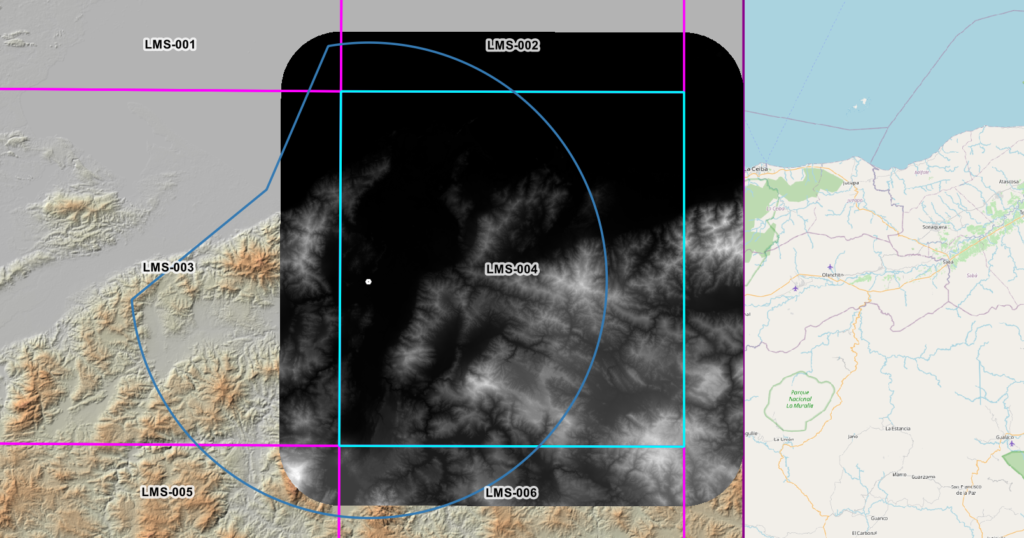
From the above image you can see our area of interest (AOI) is represented by the blue rectangle but we have 10 NM around it to account for the mountainous area distance we need to check for each raster pixel within the LMS-004 tile. We are ready now for the heavy tasks
- Run r.neighbors to get the max value within approximately 10 NM (407 pixels) save as max_LMS-004.tif
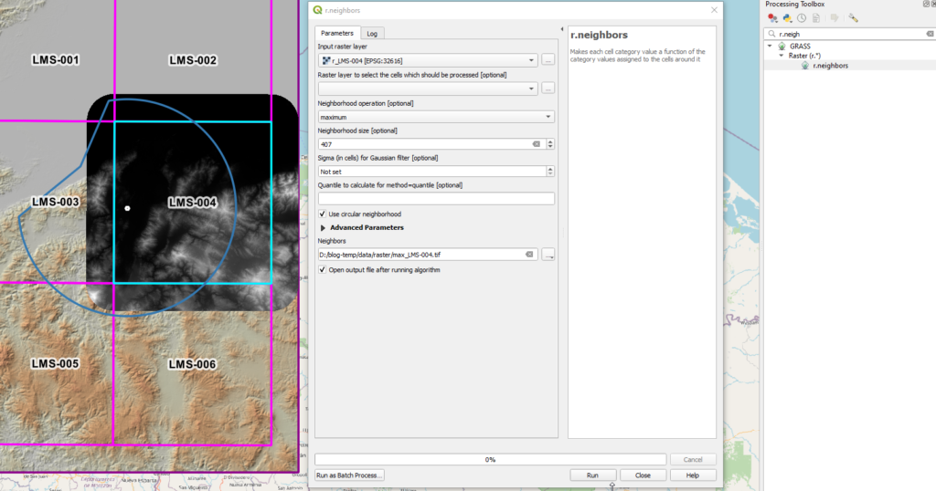
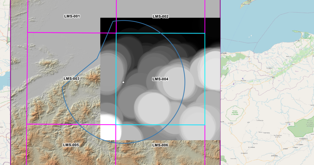
- Run r.neighbors to get the min value also with 407 value save as min_LMS-004.tif
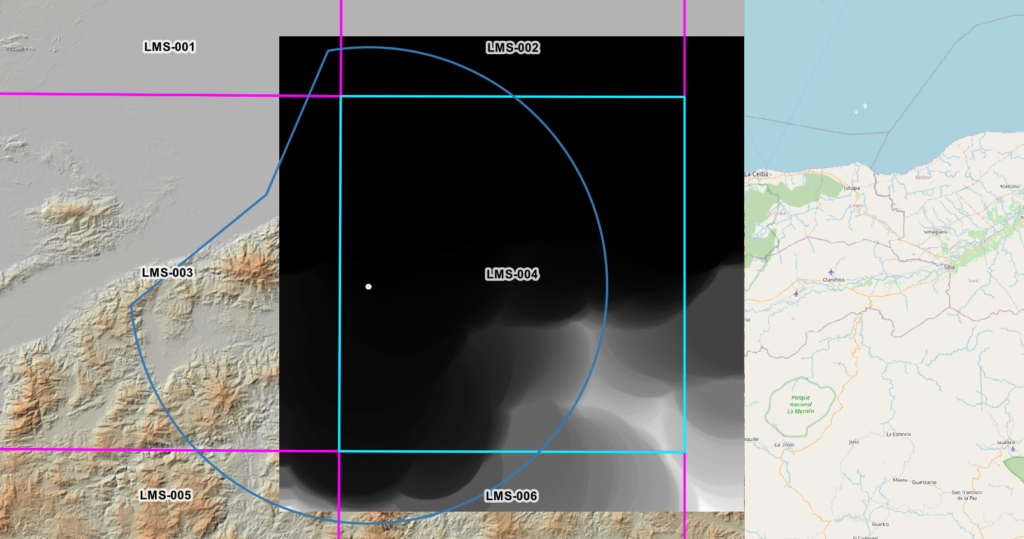
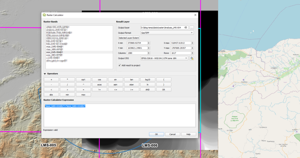
- Use the raster calculator to subtract «max_LMS-004@1»-«min_LMS-004@1» save as Analysis_LMS-004.tif
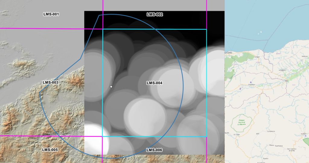
- Select value > 900 m from previous raster using the raster calculator and save as MA_LMS-004.tif
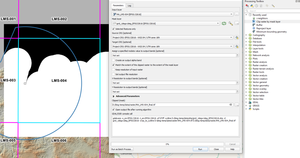
- Extract only what is in the original LMS-004 polygon as the result is only valid within it and name it MA_LMS-004_final.tif
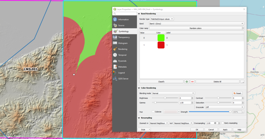
We can apply the following rendering and 50% transparency
For us the max and min neighborhood analysis took about 22 min 30 sec each, the other calculations were almost instant, so each 1degx1deg grid at this resolution can be done in roughly 45 min. Not bad at all especially considering this will be done once and the analysis will be reused.
I think you can see how the mountainous areas defined in red closely follow the edges of the mountains shown through the application of a hillshade effect which kind of validates our model visually. Of course, you could do random testing using single point analysis to do QA/QC as demonstrated in part I of this series.
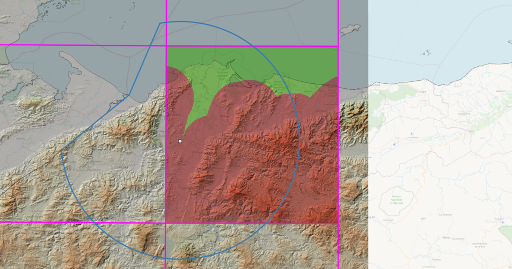
Now we need to repeat the process above for all the other relevant tiles in our area, merge them all and produce a single map from it. Keep in mind at the edges there may be small gaps that will require the voids to be filled. Once everything is in place, we can extract the filled contours if we want to represent the mountainous areas in a map
We will leave that for another blog post.
What do you think? Did you find this insightful?


0 comentarios